MILP

Here we will show how to use the naive implementation of a MILP branch and bound using scipy to solve LP of each node.

import numpy as np

from bnbprob.milpy import MILP
from bnbpy import (
    BranchAndBound,
    BreadthFirstBnB,
    plot_tree,
)

Simple model

The simple model has the form.

\[\begin{split}\begin{aligned} \text{maximize}~ \;\; & 5 x_{1} + 4 x_{2} \\ \text{subject to}~ \;\; & 2 x_{1} + 3 x_{2} \leq 12 \\ & 2 x_{1} + x_{2} \leq 6 \\ & x_{i} \geq 0 & \forall \; i \in \{ 1, 2 \} \\ & x_{i} \in \mathbb{Z} & \forall \; i \in \{ 1, 2 \} \end{aligned}\end{split}\]

# Simple problem
c = np.array([-5.0, -4.0])

A_ub = np.array(
    [[2.0, 3.0],
     [2.0, 1.0]]
)
b_ub = np.array([12.0, 6.0])

milp = MILP(c, A_ub=A_ub, b_ub=b_ub)
bfs = BreadthFirstBnB()
sol = bfs.solve(milp)
print(f"Sol: {sol} | x: {sol.problem.results.x}")

Sol: Status: OPTIMAL | Cost: -18.0 | LB: -19.5 | x: [2. 2.]

dfs = BranchAndBound()
sol = dfs.solve(milp)
print(f"Sol: {sol} | x: {sol.problem.results.x}")

Sol: Status: OPTIMAL | Cost: -18.0 | LB: -19.5 | x: [2. 2.]

Multi-dimensional knapsack

# Two-dimensional knapsack
np.random.seed(42)

N = 10  # Number of items

# Weight associated with each item
w = np.random.normal(loc=5.0, scale=1.0, size=N).clip(0.5, 10.0)
v = np.random.normal(loc=6.0, scale=2.0, size=N).clip(0.5, 10.0)

# Price associated with each item
c = -np.random.normal(loc=10.0, scale=1.0, size=N).clip(0.5, 20.0)

# knapsack capacity
kw = 21.0
kv = 22.0

A_ub = np.atleast_2d([w, v])
b_ub = np.array([kw, kv])

milp = MILP(c, A_ub=A_ub, b_ub=b_ub, bounds=(0, 1))
bnb = BranchAndBound(save_tree=True)
sol = bnb.solve(milp, maxiter=250)
print(f"Nodes explored: {bnb.explored}")
print(f"Sol: {sol} | {bnb.explored} iterations")

Nodes explored: 107
Sol: Status: OPTIMAL | Cost: -41.726493076490556 | LB: -41.726493076490556 | 107 iterations

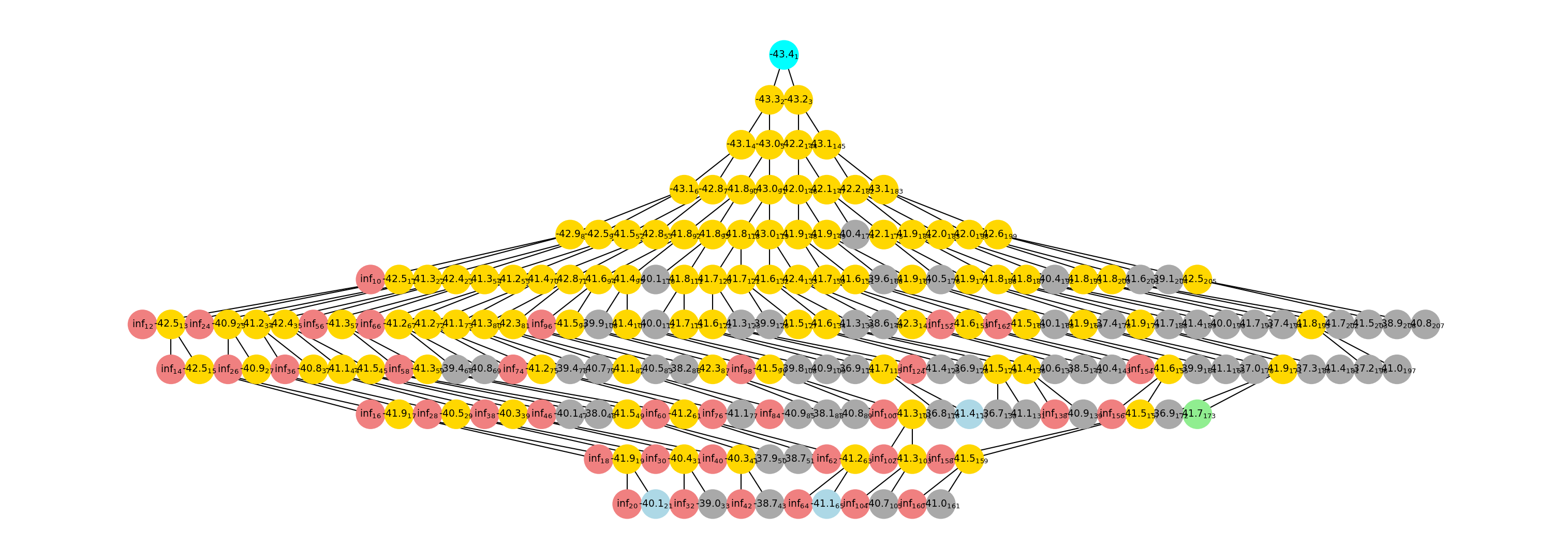
And we can plot the search tree.

plot_tree(bnb.root, font_size=9, figsize=[20, 7], dpi=150)